Week 3

Data Types

Agenda

Discussion of Assigned Reading
Intro to R and Data Cleaning
Activity
Exploratory Data Analysis

Discussion of Assigned Reading

Reading: The Persistent Grip of Social Class on College Admissions
What was the design element you liked?
How do you think grammar of graphics was portrayed in the graph?

03:00

Vectors in R

A vector is like a single column of data in R, it’s a list of values that are all the same type (like all numbers or all words).
Example:

# A vector of numbers
numbers <- c(1, 2, 3, 4, 5)

# A vector of words
fruits <- c("apple", "banana", "cherry")

# A vector of TRUE/FALSE values
logic <- c(TRUE, FALSE, TRUE)

Data Frames in R

A data frame is like a table or spreadsheet — it has rows and columns, and each column can have its own type (numbers, words, etc.).

# Create a data frame
students <- data.frame(
  name = c("Alice", "Bob", "Charlie"),
  age = c(20, 21, 19),
  major = c("Math", "Physics", "Biology")
)

# Print the data frame
print(students)

     name age   major
1   Alice  20    Math
2     Bob  21 Physics
3 Charlie  19 Biology

Data types in R

Data Types: A data type tells you what kind of data something is, like a number, a word (string), or a TRUE/FALSE value (logical).

# Numeric (numbers)
num <- 42

# Character (text)
text <- "Hello, R!"

# Logical (TRUE/FALSE)
logic <- TRUE

# Print the values and their types
print(num)      # 42

[1] 42

print(text)     # "Hello, R!"

[1] "Hello, R!"

print(logic)    # TRUE

[1] TRUE

# Check the data type using class()
class(num)   # "numeric"

[1] "numeric"

class(text)  # "character"

[1] "character"

class(logic) # "logical"

[1] "logical"

Data Cleaning

Real data has:

inconsistent labels
missing values
mixed units
impossible numbers

dplyr and tidyr are part of the tidyverse (package) and help you clean data using readable, step-by-step pipelines. Together, they make it easy to standardize values, reshape tables, handle missing data, and prepare datasets for analysis.

Functions we use to clean data

Function	What it does	Example
`str_trim()`	Remove extra spaces	`" Coffee "` → `"Coffee"`
`str_to_lower()`	Convert text to lowercase	`"Tea"` → `"tea"`
`str_to_upper()`	Convert text to uppercase	`"Water"` → `"WATER"`

Functions we use to clean data (Continued)

parse_number() extracts the first number it finds in a string.

library(tidyverse)

df <- df |>
  mutate(
    hours = parse_number(hours),
    commute = parse_number(commute),
    units = parse_number(units)
  )

Functions we use to clean data (Continued)

case_when() Creates a new variable using multiple conditions.

df <- df |>
  mutate(
    drink_clean = case_when(
      #logical condition, condition ~ value_if_true “is in”
      #If condition is TRUE, then assign "water"
      #drink == "water" checks ONE VALUE 
      drink %in% c("water", "sparkling water") ~ "water",
      drink %in% c("tea", "peach iced tea") ~ "tea",
      drink %in% c("coffee", "coffee/liquid") ~ "coffee",
      TRUE ~ "other"
    )
  )

Data Cleaning

Before we can clean data, we first need to load it into our R session.

CSVs

A comma separate value (CSV) file stores tabular data with each row on a new line and each column delimited by a comma. Good for storing R data frames in your file system.

Reading into R (base R)

data <- read.csv("data/week1_survey.csv")
data

CSVs

A comma separate value (CSV) file stores tabular data with each row on a new line and each column delimited by a comma. Good for storing R data frames in your file system.

Reading into R (`readr`)

library(readr)
# library(tidyverse) # easy alternative
# read_csv: modern tidyverse approach, faster, safer, more predictable
data <- read_csv("data/week1_survey.csv")
data

# A tibble: 19 × 7
   hours           transfer gradstudent commute   drink             major  units
   <chr>           <lgl>    <lgl>       <chr>     <chr>             <chr>  <chr>
 1 7               FALSE    FALSE       20        water             Rheto… 6    
 2 8               FALSE    FALSE       10 min    water             Env.E… 15   
 3 7 hours         TRUE     TRUE        20 mins   coffee            Busin… 13   
 4 6 hrs           TRUE     FALSE       5 min     champagne         appli… 13 u…
 5 4 hours/5 hours FALSE    FALSE       10 min    sprite            Econo… 16   
 6 9hrs            TRUE     FALSE       45 min    coffee            DATA … 13 u…
 7 7 hours         FALSE    FALSE       7 mins    water             Data … 14   
 8 6 hrs           FALSE    FALSE       ~10       Peach Iced tea    CB     18   
 9 8h              TRUE     FALSE       5m        water             Data … 14   
10 7h30            FALSE    FALSE       20 min    water             Molec… 15   
11 8h              TRUE     FALSE       60        tea               stati… 20   
12 8hours/wd       FALSE    FALSE       2 minutes coffee/liquid     legal… 17 u…
13 7.5h            FALSE    FALSE       30 min    tea               poli.… 20u  
14 7h avg          NA       TRUE        20 minute sparkling water   Buisi… 15   
15 7.5h            FALSE    TRUE        35 min    gin and tonic     stati… 13   
16 6               TRUE     FALSE       10        Tea               compu… 11   
17 8 hours         TRUE     FALSE       45 min    water             Data … 17 u…
18 6               FALSE    FALSE       20        tea               math   20   
19 6               FALSE    FALSE       10 min    Iced Matcha Latte Socio… 12

Data Cleaning (Continued)

#Preview the first few rows of the dataset
head(data)

# A tibble: 6 × 7
  hours           transfer gradstudent commute drink     major             units
  <chr>           <lgl>    <lgl>       <chr>   <chr>     <chr>             <chr>
1 7               FALSE    FALSE       20      water     Rhetoric          6    
2 8               FALSE    FALSE       10 min  water     Env.Econ          15   
3 7 hours         TRUE     TRUE        20 mins coffee    Business managem… 13   
4 6 hrs           TRUE     FALSE       5 min   champagne applied math      13 u…
5 4 hours/5 hours FALSE    FALSE       10 min  sprite    Economics         16   
6 9hrs            TRUE     FALSE       45 min  coffee    DATA SCIENCE      13 u…

Core dplyr functions

slice() # Pick rows by position (e.g., first 5 rows)
select() # Choose specific columns
filter() # Keep rows that meet a condition
mutate() # Create or modify columns
arrange() # Sort rows by one or more variables
summarize() # Compute summary statistics (mean, count, etc.)
group_by() # Group data so summaries are done per category

dplyr verbs

slice()
select()
filter()
mutate()
arrange()
summarize()
group_by()

All of these have a data frame as the first argument.
All of these produce a data frame as output.
Within the function, you can simply refer to column names unquoted.

Data Pipelines in R

2016: magrittr introduces %>%

|>

2021:

R now provides a simple native forward pipe syntax |>. The simple form of the forward pipe inserts the left-hand side as the first argument in the right-hand side call.

Using pipeline with our data

Without the pipeline, we would have to apply each function one at a time:

summarize(
  filter(data, major == "statistics"),
  mean(sleep_hours, na.rm = TRUE)
)
# results in nested function which can be very messy

Using the pipeline, this becomes very clean:

data |>
  filter(major == "statistics") |>
  summarise(mean(sleep_hours, na.rm = TRUE))

What we want:

library(tidyverse)

farm_data <- tibble(
  employee_id = 1:10,
  hours_worked = c(40, 55, 38, 60, 45, 50, 42, 65, 37, 48),
  seasonal_worker = c(TRUE, TRUE, FALSE, TRUE, FALSE, TRUE, FALSE, TRUE, FALSE, FALSE),
  supervisor = c(FALSE, FALSE, TRUE, FALSE, TRUE, FALSE, TRUE, FALSE, TRUE, FALSE),
  commute_min = c(15, 35, 20, 50, 10, 40, 25, 60, 12, 30),
  primary_crop = c("Corn", "Wheat", "Corn", "Soy",
                   "Soy", "Wheat", "Corn", "Soy",
                   "Corn", "Wheat"),
  years_experience = c(2, 5, 10, 3, 12, 4, 8, 1, 15, 6),
  hourly_wage = c(18, 20, 25, 19, 28, 21, 24, 17, 30, 23)
)

farm_data

# A tibble: 10 × 8
   employee_id hours_worked seasonal_worker supervisor commute_min primary_crop
         <int>        <dbl> <lgl>           <lgl>            <dbl> <chr>       
 1           1           40 TRUE            FALSE               15 Corn        
 2           2           55 TRUE            FALSE               35 Wheat       
 3           3           38 FALSE           TRUE                20 Corn        
 4           4           60 TRUE            FALSE               50 Soy         
 5           5           45 FALSE           TRUE                10 Soy         
 6           6           50 TRUE            FALSE               40 Wheat       
 7           7           42 FALSE           TRUE                25 Corn        
 8           8           65 TRUE            FALSE               60 Soy         
 9           9           37 FALSE           TRUE                12 Corn        
10          10           48 FALSE           FALSE               30 Wheat       
# ℹ 2 more variables: years_experience <dbl>, hourly_wage <dbl>

Reality with data

farm_raw <- tibble(
  employee_id = 1:6,
  hours_worked = c("40 hours", "55 hrs", "38 hrs", "60 hours", "45hrs", "50hours"),
  seasonal_worker = c("yes", "TRUE", "no", "Yes", "false", "TRUE"),
  supervisor = c("no", "no", "TRUE", "no", "TRUE", "no"),
  commute_min = c("15 minutes", "35 mins", "20min", "50 minute", "10minutes", "40mins"),
  primary_crop = c(" Corn", "wheat ", "CORN", "Soy", " soy ", "WHEAT"),
  years_experience = c("2 years", "5rs", "10 yrs", "3 yr", "12 years", "4yr"),
  hourly_wage = c("18 dollars", "20/hr", "25 per hour", "19 dollars", "28 usd", "21 /day")
)

Data Cleaning Example:

library(tidyverse)

farm_clean <- farm_raw |>
  mutate(
    # numeric columns
    hours_worked = parse_number(hours_worked),
    commute_min = parse_number(commute_min),
    years_experience = parse_number(years_experience),
    hourly_wage = parse_number(hourly_wage),

    # yes/no variables
    seasonal_worker = case_when(
      str_to_lower(str_trim(seasonal_worker)) %in% c("yes", "true") ~ TRUE,
      str_to_lower(str_trim(seasonal_worker)) %in% c("no", "false") ~ FALSE,
      TRUE ~ NA
    ),

    supervisor = case_when(
      str_to_lower(str_trim(supervisor)) %in% c("yes", "true") ~ TRUE,
      str_to_lower(str_trim(supervisor)) %in% c("no", "false") ~ FALSE,
      TRUE ~ NA
    ),

    # categorical cleanup
    primary_crop =
      primary_crop |>
      str_trim() |>
      str_to_lower()
  )

farm_clean

# A tibble: 6 × 8
  employee_id hours_worked seasonal_worker supervisor commute_min primary_crop
        <int>        <dbl> <lgl>           <lgl>            <dbl> <chr>       
1           1           40 TRUE            FALSE               15 corn        
2           2           55 TRUE            FALSE               35 wheat       
3           3           38 FALSE           TRUE                20 corn        
4           4           60 TRUE            FALSE               50 soy         
5           5           45 FALSE           TRUE                10 soy         
6           6           50 TRUE            FALSE               40 wheat       
# ℹ 2 more variables: years_experience <dbl>, hourly_wage <dbl>

Activity:

Download your data from the CSV in BCourses
Download the .qmd file which has the instructions
Open the .qmd file in Positron or RStudio
Clean all columns to respective datatype

20:00

Exploratory Data Analysis

After having cleaned the data, we want to get a sense of what we are looking at.

Let’s use our farm_data data as an example.

Q1: What are the cols and rows?

dim(farm_data)

[1] 10  8

sapply(farm_data, class)

     employee_id     hours_worked  seasonal_worker       supervisor 
       "integer"        "numeric"        "logical"        "logical" 
     commute_min     primary_crop years_experience      hourly_wage 
       "numeric"      "character"        "numeric"        "numeric"

Q1: What are the cols and rows?

farm_data

# A tibble: 10 × 8
   employee_id hours_worked seasonal_worker supervisor commute_min primary_crop
         <int>        <dbl> <lgl>           <lgl>            <dbl> <chr>       
 1           1           40 TRUE            FALSE               15 Corn        
 2           2           55 TRUE            FALSE               35 Wheat       
 3           3           38 FALSE           TRUE                20 Corn        
 4           4           60 TRUE            FALSE               50 Soy         
 5           5           45 FALSE           TRUE                10 Soy         
 6           6           50 TRUE            FALSE               40 Wheat       
 7           7           42 FALSE           TRUE                25 Corn        
 8           8           65 TRUE            FALSE               60 Soy         
 9           9           37 FALSE           TRUE                12 Corn        
10          10           48 FALSE           FALSE               30 Wheat       
# ℹ 2 more variables: years_experience <dbl>, hourly_wage <dbl>

Q1: What are the cols and rows?

Unit of observation: an individual farm worker
Variables: employee ID (integer), hours worked (numeric), seasonal worker (logical), supervisor (logical), commute in minutes (numeric), primary crop (character), years of experience (numeric), hourly wage (numeric)

A description of the variables is often stored in a separate file called a data dictionary.

Q2: Is there any missing data?

Option 1: Total missing values

library(dplyr)
sum(is.na(farm_data))

[1] 0

Option 2: Proportion missing counts

farm_data |>
  summarize(across(everything(), ~ mean(is.na(.))))

# A tibble: 1 × 8
  employee_id hours_worked seasonal_worker supervisor commute_min primary_crop
        <dbl>        <dbl>           <dbl>      <dbl>       <dbl>        <dbl>
1           0            0               0          0           0            0
# ℹ 2 more variables: years_experience <dbl>, hourly_wage <dbl>

Q3: What is the distribution of `years_experience`?

library(ggplot2)
farm_data |>
  ggplot(aes(x = years_experience)) +
  geom_bar()

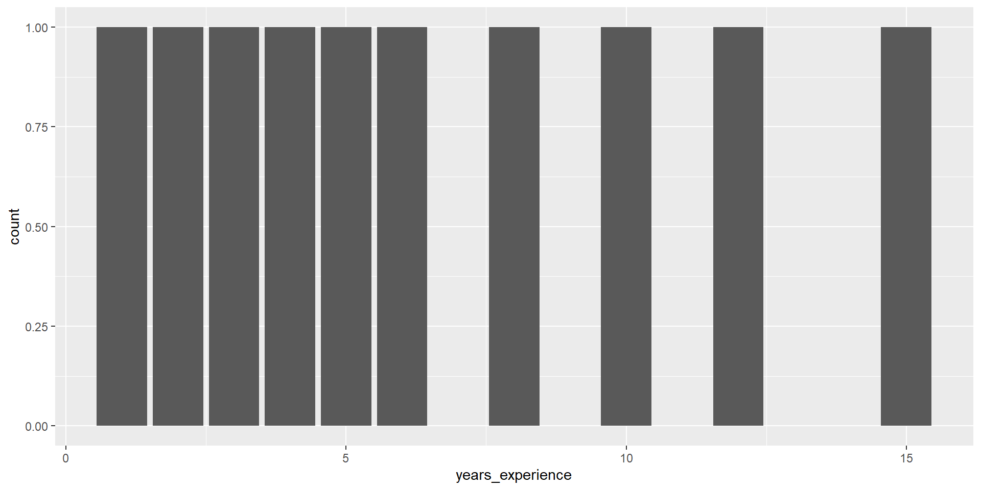
Q3: What is the distribution of `years_experience`?

farm_data |>
  ggplot(aes(y = years_experience)) +
  geom_bar()

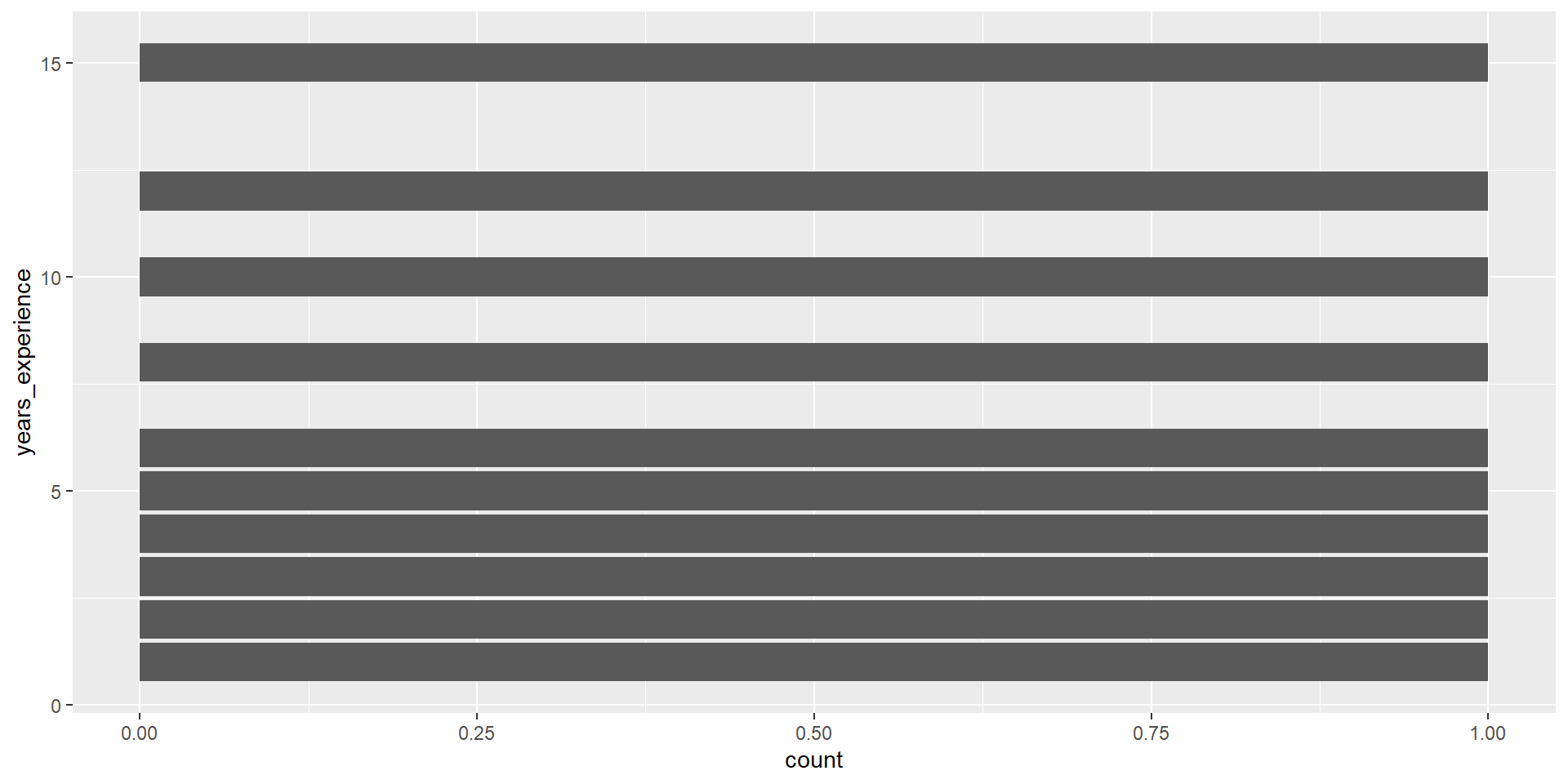
`geom_bar()`

geom_bar() counts up the number of observations in each level of a single variable, then draws bars up to that height.

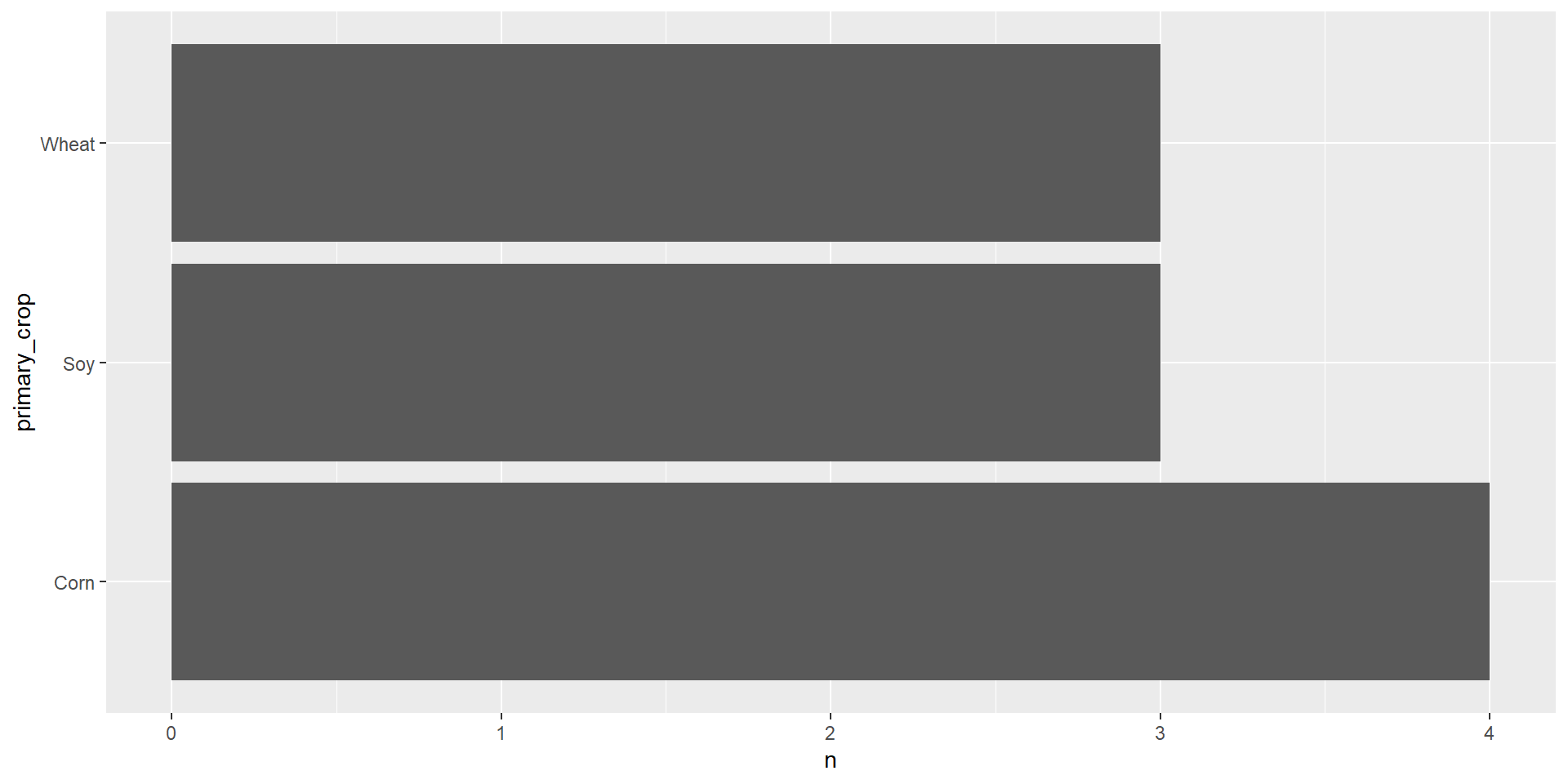
Summarizing with counts

farm_data |>
  group_by(primary_crop) |>
  summarize(count = n())

# A tibble: 3 × 2
  primary_crop count
  <chr>        <int>
1 Corn             4
2 Soy              3
3 Wheat            3

`geom_col()`

geom_col() takes one column of categories and draws a bar for each up to the height of a second column of counts.

farm_data |>
  count(primary_crop) |>
  ggplot(aes(y = primary_crop, x = n)) +
  geom_col()

Two types of Viz

Exploratory Data Analysis (EDA)

Explanatory Data Analysis

Let us know if you have any questions!

Homework 1 is posted to BCourses

Due Monday, March 2nd at 11:59PM

Reading for next week: Price of Eggs

https://www.nytimes.com/2023/02/03/briefing/why-eggs-cost-so-much.html

Week 3

Agenda

Discussion of Assigned Reading

Vectors in R

Data Frames in R

Data types in R

Data Cleaning

Functions we use to clean data

Functions we use to clean data (Continued)

Functions we use to clean data (Continued)

Data Cleaning

CSVs

Reading into R (base R)

CSVs

Reading into R (readr)

Data Cleaning (Continued)

Core dplyr functions

dplyr verbs

Data Pipelines in R

Using pipeline with our data

What we want:

Reality with data

Data Cleaning Example:

Activity:

Exploratory Data Analysis

Q1: What are the cols and rows?

Q1: What are the cols and rows?

Q1: What are the cols and rows?

Q2: Is there any missing data?

Q3: What is the distribution of years_experience?

Q3: What is the distribution of years_experience?

geom_bar()

Summarizing with counts

geom_col()

Two types of Viz

Exploratory Data Analysis (EDA)

Explanatory Data Analysis

Let us know if you have any questions!

Reading into R (`readr`)

Q3: What is the distribution of `years_experience`?

Q3: What is the distribution of `years_experience`?

`geom_bar()`

`geom_col()`